pyharmonics

pyharmonics detects harmonic patterns in OHLC candle data for any stock or crypto asset. To learn more about harmonic patterns goto http://www.harmonictrader.com and follow Scott Carney. In short, when a stock or crypto asset begins a price run ( moons ) the start point to the peak is considered 100% of the move. If the price drops and the amount it drops by is equal to 61.8%, 78.6% or 88.6% of the original pump, there is astrong chance a bottom will form and the price will recover.

This can happen and is respected on any time frame from 1 min to 1 month. To know which level the price might bottom at you need to know the ABC portion of the move. This usually involves the highest and second highest prices IF those prices peaks have a dip between them that is between 38.2% - 50% of the first pump.

See Scott Carney’s Harmonic Trader books and website for more info. There are many patterns and pyharmonics can detect them all. It can state whether a pattern is formed or forming and it can plot those patterns.

In a pyharmonics plot.

  1. Bullish patterns that have fully formed are green, bullish patterns that are still forming are yellow.

  2. Bearish patterns that have fully formed are red, bearish patterns that are still forming are purple.

Warning

pyharmonics is not financial advice. It is a tool for detecting harmonic price levels or indicator divergences for an assets price trend. Any decision taken to enter a trade on any asset is entirely yours. No risk is assumed by this API.

Installation

pip install pyharmonics

Quick Guide

>>> from pyharmonics.quick import *

This gives you.

from pyharmonics.marketdata import YahooCandleData, BinanceCandleData, YahooOptionData
from pyharmonics.technicals import OHLCTechnicals, Technicals
from pyharmonics.search import HarmonicSearch, DivergenceSearch
from pyharmonics.positions import Position
from pyharmonics.plotter import HarmonicPlotter, PositionPlotter, OptionPlotter
from pyharmonics import constants

You also get some quick functions for plot/displaying the current status of a asset.

whats_new_binance(symbol, interval, limit_to=-1, candles=1000)
whats_new_yahoo(symbol, interval, limit_to=-1, candles=1000)

See every ABC, ABCD and XABCD pattern that has formed on an asset. set limit_to=3 to see patterns that completed within the last 3 peaks ( recommended )

whats_forming_binance(symbol, interval, limit_to=10, percent_complete=0.8, candles=1000)
whats_forming_yahoo(symbol, interval, limit_to=10, percent_complete=0.8, candles=1000)

See every ABC, ABCD and XABCD pattern that is forming on an asset. set limit_to=3 to see patterns that completed within the last 3 peaks ( recommended )

whats_options_volume(symbol)
whats_options_interest(symbol)

plots options open interest or volume for a stock. This is very useful as it shows where the writer of the options needs the price to move to in order to limite their losses!

Market data

pyharmonics requires pandas DataFrame objects. You can create your own. The schema required is shown below. Pyharmonics can extract market data from Binance, Yahoo and Alpaca ( more to come ).

 1>>> from pyharmonics.marketdata import YahooCandleData
 2>>> y = YahooCandleData()
 3>>> y.get_candles('MSFT', y.MIN_5, 300)
 4>>> y.df
 5                                open        high       close       close  volume
 6index
 72023-07-06 18:15:00+01:00  342.410004  342.880005  342.858093  342.858093  299423
 82023-07-06 18:20:00+01:00  342.859985  342.989990  342.825012  342.825012  186800
 92023-07-06 18:25:00+01:00  342.829987  342.829987  342.029999  342.029999  253544
102023-07-06 18:30:00+01:00  342.045013  342.109985  341.720001  341.720001  236668
112023-07-06 18:35:00+01:00  341.779907  342.140015  342.089996  342.089996  190417
12...                               ...         ...         ...         ...     ...
132023-07-12 16:50:00+01:00  336.829987  336.869995  336.390015  336.390015  345811
142023-07-12 16:55:00+01:00  336.369995  336.625000  336.429993  336.429993  301966
152023-07-12 17:00:00+01:00  336.435486  337.154999  336.839996  336.839996  264732
162023-07-12 17:05:00+01:00  336.829987  336.899994  336.684998  336.684998  200605
172023-07-12 17:10:00+01:00  336.690002  337.229004  337.059998  337.059998  110316
18
19[300 rows x 5 columns]
20>>>

All candle data classes support MIN_1, MIN_5, MIN_15, HOUR_1, DAY_1, WEEK_1, MONTH_1, MONTH_3 time horizons. BinanceCandleData and AplacaCandleData also support HOUR_2, HOUR_4, HOUR_8, MIN_3. You can use any time frame you want. You will need to supply this information later if you want to plot meaningfully.

CandleData that requires api keys.

1>>> from pyharmonics.marketdata import AlpacaCandleData
2>>> key = dict('api'='whatever', 'secret'='whatever')
3>>> a = AlpacaCandleData(key)
4>>> a.get_candles('QQQ', y.MIN_5, 300)

Alpaca requires a dictionary with both a key and secret. Binance and Yahoo do not. Binance can accept an API key if you have created one. Order placement on any API requires a KEY but is not covered by this API.

Warning

If you are supplying a key to any API endpoint please store those keys safely and never ever commit them accidentally to any repo. Your keys are your account. Losing control of them is losing control of your account.

Binance Usage:

 1>>> from pyharmonics.marketdata import BinanceCandleData
 2>>> b = BinanceCandleData()
 3>>> b.get_candles('ETHUSDT', b.MIN_5, 300)
 4>>> b.df
 5
 6                              open     high      low    close     volume  close_time                       dts
 7index
 82023-09-12 10:04:59+01:00  1577.85  1578.82  1577.85  1578.07   778.5332  1694509499 2023-09-12 10:04:59+01:00
 92023-09-12 10:09:59+01:00  1578.07  1578.32  1577.16  1577.34   283.1288  1694509799 2023-09-12 10:09:59+01:00
102023-09-12 10:14:59+01:00  1577.35  1578.15  1576.38  1577.90   525.5365  1694510099 2023-09-12 10:14:59+01:00
112023-09-12 10:19:59+01:00  1577.91  1580.58  1577.90  1579.66   742.6356  1694510399 2023-09-12 10:19:59+01:00
122023-09-12 10:24:59+01:00  1579.67  1580.28  1579.09  1579.42   622.7093  1694510699 2023-09-12 10:24:59+01:00
13...                            ...      ...      ...      ...        ...         ...                       ...
142023-09-13 10:39:59+01:00  1597.73  1600.48  1596.59  1599.01  1818.5411  1694597999 2023-09-13 10:39:59+01:00
152023-09-13 10:44:59+01:00  1599.01  1600.91  1597.32  1598.05  1119.4597  1694598299 2023-09-13 10:44:59+01:00
162023-09-13 10:49:59+01:00  1598.05  1598.35  1596.95  1597.11   499.6893  1694598599 2023-09-13 10:49:59+01:00
172023-09-13 10:54:59+01:00  1597.12  1600.47  1597.11  1600.30   573.2835  1694598899 2023-09-13 10:54:59+01:00
182023-09-13 10:59:59+01:00  1600.30  1602.44  1598.80  1600.20  2461.2631  1694599199 2023-09-13 10:59:59+01:00

Using the OHLCTechnicals object on OHLC Data

>>> from pyharmonics.marketdata import BinanceCandleData
>>> from pyharmonics.technicals import OHLCTechnicals
>>> b = BinanceCandleData()
>>> t = OHLCTechnicals(b.df, b.symbol, b.interval, peak_spacing=20)
Traceback (most recent call last):
File "<stdin>", line 1, in <module>
File "/home/xual/Software/pyharmonics/src/pyharmonics/technicals.py", line 129, in __init__
    raise ValueError('Candle DataFrame is None! call cd.get_candles(ASSET, INTERVAL) first.')
ValueError: Candle DataFrame is None! call cd.get_candles(ASSET, INTERVAL) first.

Note

Always remember to get candle data :-)

>>> b.get_candles('ETHUSDT', b.HOUR_4, 400)
>>> b.df
                            open     high      low    close      volume  close_time                       dts
index
2023-05-13 08:59:59+01:00  1805.62  1806.84  1796.80  1802.98  30365.3283  1683964799 2023-05-13 08:59:59+01:00
2023-05-13 12:59:59+01:00  1802.98  1811.46  1801.24  1803.78  29164.0211  1683979199 2023-05-13 12:59:59+01:00
2023-05-13 16:59:59+01:00  1803.79  1809.91  1785.23  1795.90  46713.5684  1683993599 2023-05-13 16:59:59+01:00
2023-05-13 20:59:59+01:00  1795.91  1806.45  1786.12  1792.83  40715.0401  1684007999 2023-05-13 20:59:59+01:00
2023-05-14 00:59:59+01:00  1792.84  1804.89  1792.38  1795.11  24692.1556  1684022399 2023-05-14 00:59:59+01:00
...                            ...      ...      ...      ...         ...         ...                       ...
2023-07-18 04:59:59+01:00  1911.21  1917.19  1906.25  1908.88  19832.6141  1689652799 2023-07-18 04:59:59+01:00
2023-07-18 08:59:59+01:00  1908.88  1911.72  1893.36  1898.99  37921.2814  1689667199 2023-07-18 08:59:59+01:00
2023-07-18 12:59:59+01:00  1898.99  1909.64  1890.80  1894.15  39215.5098  1689681599 2023-07-18 12:59:59+01:00
2023-07-18 16:59:59+01:00  1894.15  1903.66  1885.08  1897.20  49833.1236  1689695999 2023-07-18 16:59:59+01:00
2023-07-18 20:59:59+01:00  1897.21  1903.58  1875.73  1891.50  46447.8182  1689710399 2023-07-18 20:59:59+01:00

[400 rows x 7 columns]
>>> t = Technicals(b.df, b.symbol, b.interval)
>>> t.df
                            open     high      low    close      volume  close_time  ... price_peaks  price_dips  macd_peaks  macd_dips  rsi_peaks  rsi_dips
index                                                                                  ...
2023-05-13 08:59:59+01:00  1805.62  1806.84  1796.80  1802.98  30365.3283  1683964799  ...           0           0           0          0          0         0
2023-05-13 12:59:59+01:00  1802.98  1811.46  1801.24  1803.78  29164.0211  1683979199  ...           0           0           0          0          0         0
2023-05-13 16:59:59+01:00  1803.79  1809.91  1785.23  1795.90  46713.5684  1683993599  ...           0           0           0          0          0         0
2023-05-13 20:59:59+01:00  1795.91  1806.45  1786.12  1792.83  40715.0401  1684007999  ...           0           0           0          0          0         0
2023-05-14 00:59:59+01:00  1792.84  1804.89  1792.38  1795.11  24692.1556  1684022399  ...           0           0           0          0          0         0
...                            ...      ...      ...      ...         ...         ...  ...         ...         ...         ...        ...        ...       ...
2023-07-18 04:59:59+01:00  1911.21  1917.19  1906.25  1908.88  19832.6141  1689652799  ...           0           0           0          0          0         0
2023-07-18 08:59:59+01:00  1908.88  1911.72  1893.36  1898.99  37921.2814  1689667199  ...           0           0           0          0          0         0
2023-07-18 12:59:59+01:00  1898.99  1909.64  1890.80  1894.15  39215.5098  1689681599  ...           0           0           0          0          0         0
2023-07-18 16:59:59+01:00  1894.15  1903.66  1885.08  1897.20  49833.1236  1689695999  ...           0           0           0          0          0         0
2023-07-18 20:59:59+01:00  1897.21  1903.58  1875.73  1891.50  46447.8182  1689710399  ...           0           0           0          0          0         0

[400 rows x 27 columns]

Peak sensitivity can be increased like so.

>>> t = Technicals(b.df, peak_spacing=12)

Note

More peaks will mean more points to search through when looking for harmonic patterns. In some cases this can lead to too many patterns being identified.

Using the standard Technicals object on single trend data

>>> from pyharmonics.technicals import Technicals
>>> from pyharmonics.utils import UER
>>> t = Technicals(UER, 'Unemployment', 'monthly', peak_spacing=6)
>>> t.df
        year  close  price_peaks  price_dips      macd        rsi  stoch_rsi  ...    ema 21    ema 34    ema 55  macd_peaks  macd_dips  rsi_peaks  rsi_dips
0    2013-01-01    8.0            1           0       NaN        NaN        NaN  ...       NaN       NaN       NaN           0          0          0         0
1    2013-02-01    7.7            0           0       NaN        NaN        NaN  ...       NaN       NaN       NaN           0          0          0         0
2    2013-03-01    7.5            0           0       NaN        NaN        NaN  ...       NaN       NaN       NaN           0          0          0         0
3    2013-04-01    7.6            0           0       NaN        NaN        NaN  ...       NaN       NaN       NaN           0          0          0         0
4    2013-05-01    7.5            0           0       NaN        NaN        NaN  ...       NaN       NaN       NaN           0          0          0         0
..          ...    ...          ...         ...       ...        ...        ...  ...       ...       ...       ...         ...        ...        ...       ...
122  2023-03-01    3.5            0           0  0.036866  38.289828   0.591382  ...  4.069905  4.441627  4.740887           0          0          0         0
123  2023-04-01    3.4            0           1  0.042426  37.160633   0.686581  ...  4.009005  4.382106  4.692998           0          0          0         0
124  2023-05-01    3.7            1           0  0.068006  42.627002   0.736196  ...  3.980914  4.343128  4.657534           0          0          1         0
125  2023-06-01    3.6            0           0  0.079110  41.336196   0.769141  ...  3.946285  4.300664  4.619765           0          0          0         0
126  2023-07-01    3.5            0           0  0.080380  40.030762   0.794174  ...  3.905714  4.254912  4.579774           1          0          0         0

[127 rows x 22 columns]

Technicals.df schema

>>> t.df.columns
Index(['open', 'high', 'low', 'close', 'volume', 'close_time', 'dts', 'macd',
    'rsi', 'stoch_rsi', 'bb%', 'sma 50', 'sma 100', 'sma 150', 'sma 200',
    'ema 5', 'ema 8', 'ema_13', 'ema 21', 'ema 34', 'ema 55', 'price_peaks',
    'price_dips', 'macd_peaks', 'macd_dips', 'rsi_peaks', 'rsi_dips'],
    dtype='object')
  • `'macd', 'rsi', 'stoch_rsi', 'bb%'` are the MACD ( Moving Avg. Convergence Divergence ), RSI ( Relative strength index ), Stochastic RSI and Bollinger Band deviation reading.

  • `'sma 50', 'sma 100', 'sma 150', 'sma 200'` are Simple Moving Avergaes SMA. 50, 100, 150, 200 candle average. All useful for plotting support/resistance levels.

  • `'ema 5', 'ema 8', 'ema_13', 'ema 21', 'ema 34', 'ema 55'` are Exponential moving averages all fibonacci numbers. Very accurate in plotting support/resistance as swings move.

  • `'price_peaks', 'price_dips', 'macd_peaks', 'macd_dips', 'rsi_peaks', 'rsi_dips'` the indexes where the price is at a peak or dip. Similar for the MACD and RSI. This informatoin is key for detecting divergence patterns which confirm harmonic patterns.

Harmonic Searches

Harmonic searches are searches for ABC, ABCD or XABCD patterns. On the final point of the pattern a price reversal is more likely to occur. The MatrixSearch object performs this search using a very efficent algorithm. A brute force 5 point search would constitute

\[complexity = O(n-m)^5\]

1000 candles with n = 100 peaks would consitiute a 100*99*98*97*96 search with 9034502400 passes!!

MatrixSearch is

\[complexity = O(n^2/2 + (n-m)^2/2)\]

where

\[n\2 <= m <= n\]

1000 candles with n = 100 peaks consitiutes a 100^2/2 ( lower triangle ) scan followed by an additional (n-m)^2/2 loops to link patterns. That’s 5000 + 1250 passes to locate all patterns in the dataframe. That is 1445520 times faster than brute force.

Note

It implies that instead of scanning one Asset in 30 seconds using a brute force approach you can now scan 1.446 Millions assets in the same 30 seconds. The internet is now the slowest part of this problem.

 1>>> from pyharmonics.marketdata import BinanceCandleData
 2>>> from pyharmonics.search import MatrixSearch
 3>>> from pyharmonics.technicals import Technicals
 4>>> b = BinanceCandleData()
 5>>> b.get_candles('ETHUSDT', b.HOUR_4, 400)
 6>>> t = Technicals(b.df, b.symbol, b.interval)
 7>>> m = MatrixSearch(t)
 8>>> m.search()
 9>>> patterns = m.get_patterns()
10>>> patterns[m.XABCD]
11[]
12>>> patterns[m.ABCD]
13[ABCDPattern(name='ABCD-50-1.618', formed=True, retraces={'ABC': 0.5000347246336551, 'BCD': 3.31138888888889, 'ABCD': 3.31138888888889}, bullish=False, x=[Timestamp('2023-06-15 12:59:59+0100', tz='Europe/Dublin'), Timestamp('2023-06-17 08:59:59+0100', tz='Europe/Dublin'), Timestamp('2023-06-19 20:59:59+0100', tz='Europe/Dublin'), Timestamp('2023-06-23 20:59:59+0100', tz='Europe/Dublin')], y=[1626.01, 1770.0, 1698.0, 1936.42], abc_extensions=[1936.42], completion_min_price=1930.992, completion_max_price=1930.992)]
14>>> patterns[m.ABCD][0]
15ABCDPattern(name='ABCD-50-1.618', formed=True, retraces={'ABC': 0.5000347246336551, 'BCD': 3.31138888888889, 'ABCD': 3.31138888888889}, bullish=False, x=[Timestamp('2023-06-15 12:59:59+0100', tz='Europe/Dublin'), Timestamp('2023-06-17 08:59:59+0100', tz='Europe/Dublin'), Timestamp('2023-06-19 20:59:59+0100', tz='Europe/Dublin'), Timestamp('2023-06-23 20:59:59+0100', tz='Europe/Dublin')], y=[1626.01, 1770.0, 1698.0, 1936.42], abc_extensions=[1936.42], completion_min_price=1930.992, completion_max_price=1930.992)
16>>> patterns[m.ABC][0]
17ABCPattern(name=0.382, formed=True, retraces={'ABC': 0.386628628131977}, bullish=True, x=[Timestamp('2023-06-15 12:59:59+0100', tz='Europe/Dublin'), Timestamp('2023-07-14 04:59:59+0100', tz='Europe/Dublin'), Timestamp('2023-07-17 20:59:59+0100', tz='Europe/Dublin')], y=[1626.01, 2029.11, 1873.26], abc_extensions=[1873.26], completion_min_price=1873.26, completion_max_price=1873.26)
18>>>

Here we can see a single ABCD pattern formed on ETHUSDT. Its completion time was Timestamp('2023-06-23 20:59:59+0100', tz='Europe/Dublin'). Data can be specifically referenced from the pattern object.

1>>> p = patterns[m.ABC][0]
2>>> p.name
30.382
4>>> p.x
5[Timestamp('2023-06-15 12:59:59+0100', tz='Europe/Dublin'), Timestamp('2023-07-14 04:59:59+0100', tz='Europe/Dublin'), Timestamp('2023-07-17 20:59:59+0100', tz='Europe/Dublin')]
6>>> p.y
7[1626.01, 2029.11, 1873.26]
8>>>

As you can no doubt tell this information can be plotted with b.df to show you where the pattern is on the chart.

Plotting

You can plot any technicals object ( OHLCTechnicals or Technicals) using a basic Plotter or position Plotter.

Plotting is not a function added to technicals because it should not be part of that object. The plotters provided are basic but sufficent for testing and feedback.

Plot the findings.

>>> from pyharmonics.plotter import Plotter
>>> p = Plotter(t, 'BTCUSDT', b.HOUR_1)
>>> p.add_matrix_plots(m.get_patterns(family=m.XABCD))
>>> p.show()

You will see something like this.

Fully formed patterns

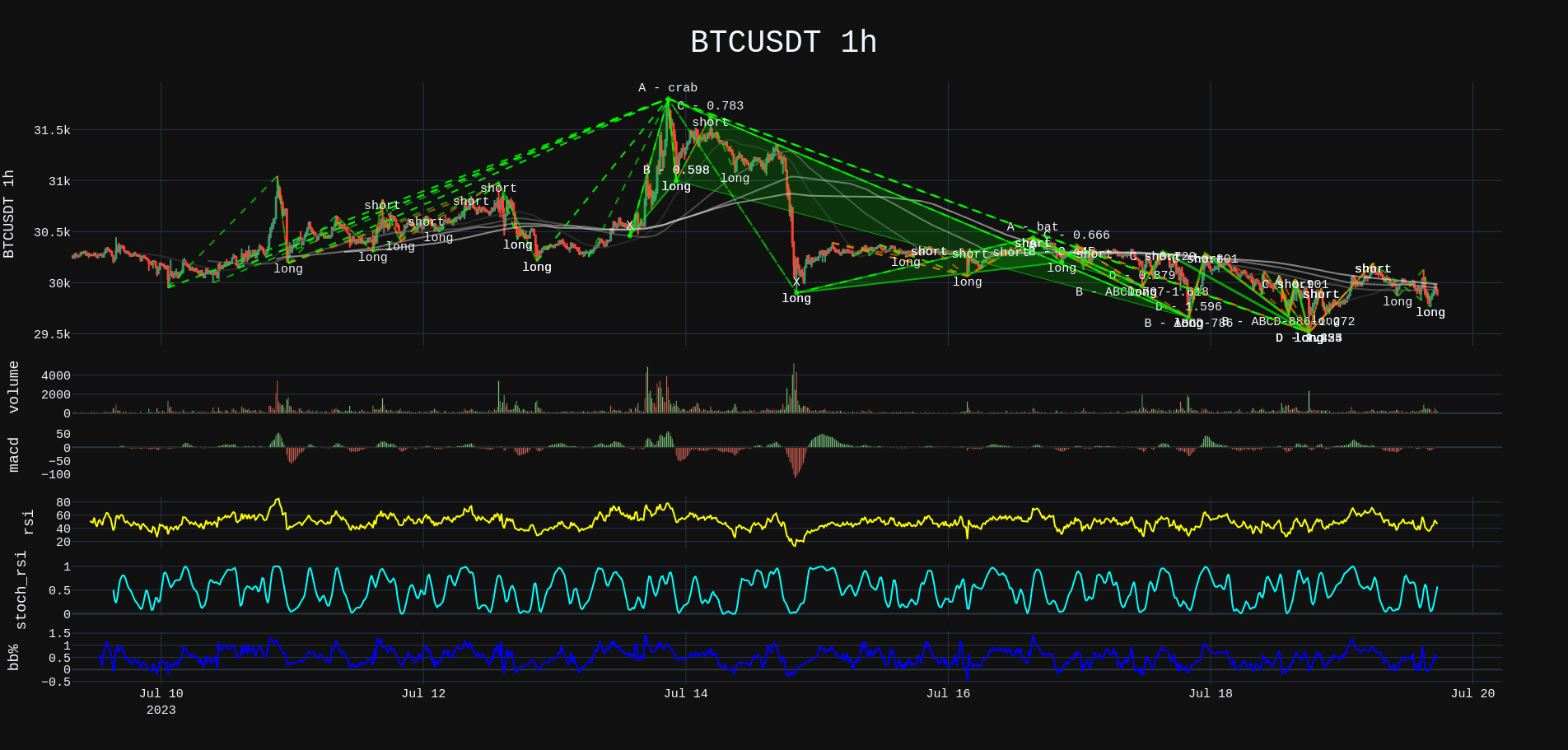
See all harmonic patterns.

>>> p = Plotter(t, 'BTCUSDT', b.HOUR_1)
>>> p.add_matrix_plots(m.get_patterns())
>>> p.show()

You will see something like this.

Fully formed patterns

See all forming patterns.

>>> m = MatrixSearch(t)
>>> m.forming()
>>> p = Plotter(t, 'BTCUSDT', b.HOUR_1)
>>> p.add_matrix_plots(m.get_patterns(formed=False))
>>> p.show()

Position add_matrix_plots

>>> m = MatrixSearch(t)
>>> m.search()
>>> patterns = m.get_patterns(family=m.XABCD)
>>> pattern = patterns[m.XABCD][0]
>>> # After extracting a pattern in isolation a position can be created.
>>> # Position(pattern, symbol, interval, strike_price, dollar_amount)
>>> position = Position(pattern, 'BTSUSDT', b.HOUR_1, pattern.y[-1], 1000)
>>> p = PositionPlotter(t, position)
>>> p.show()

The most useful plot feature is the position plot.

A tradable position.

What is the position plot telling?

There is a bearish pattern ( butterfly ). The XAB leg of the price move was a .786 ( in tolerance ) move. The ABC move was between .382 and .886. The final XAD move was 1.27. Sure enough at the price level there was a reaction and so the instruction is to set a price target at the confirmation price level.

The entry or strike price is $21085. If a $1000 dollar amount is entered at this price level then the entire position is divided into 3 even parts.

  • Target 1 is usually 50% of the CD leg move.

  • The stop should be 1/3 of your target one move.

  • Target 2 is the C point on the pattern.

  • Target 3 is 1.618 times the cd leg.

The position is divided into 3 parts Pos1 Pos2 Pos3.

  1. Pos1, Pos2, Pos3 will all close witha STOP if the price hits 21490 at a loss of -1.88%. This protects your account if the pattern does not play out.

  2. Pos1, also close with a LIMIT at $19867 locking in a 21$ profit. Pos2 and pos3 could still stop out but overall you are up $6.66

  3. Pos2, can close if the price reaches $18650 BEFORE it hits the STOP price. Pos3 could still stop out leaving you with $51.45 profit.

  4. Finally if all 3 targets hit, you make $120 profit on the initial $1000 investment. 12% is not bad.

The %Move column in the plot beside the price column indicates the size of the move. You don’t get 18% profits with that move because you sold out along the way as a risk management strategy.

Call/Put Option Plots

>>> from pyharmonics.marketdata import YahooOptionData
>>> from pyharmonics.plotter import OptionPlotter

>>> yo = YahooOptionData('NVDA')
>>> yo.analyse_options(trend='volume')
>>> p = OptionPlotter(yo, yo.ticker.options[0])
>>> p.show()

>>> yo.analyse_options(trend='openInterest')
>>> p = OptionPlotter(yo, yo.ticker.options[0])
>>> p.show()

The trend or measure for your options activity can be volume or openInterest. The OptionPlotter takes a YahooOptionsData object and an expiry date for any plot.

Although the expiry dates are present in the YahooOptionsData object you must specifically select one to view.

Options by volume

Note

volume or openInterest data resets daily. No activity for a trading can present false points of mimimum pain. Option plots are most complete by end of trading day (usually 16:30 EST)