Plotting

You can plot any technicals object ( OHLCTechnicals or Technicals) using a basic Plotter or position Plotter.

Plotting is not a function added to technicals because it should not be part of that object. The plotters provided are basic but sufficent for testing and feedback.

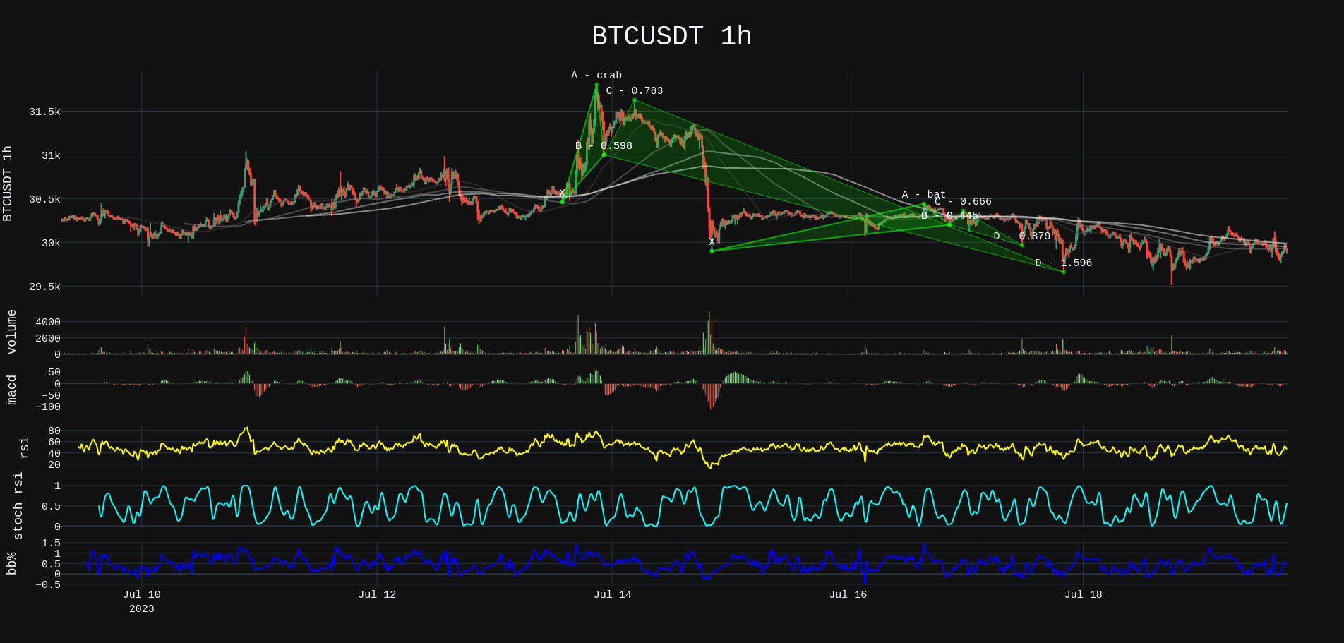
Plot the findings.

>>> from pyharmonics.plotter import Plotter
>>> p = Plotter(t, 'BTCUSDT', b.HOUR_1)
>>> p.add_harmonic_plots(m.get_patterns(family=m.XABCD))
>>> p.show()

You will see something like this.

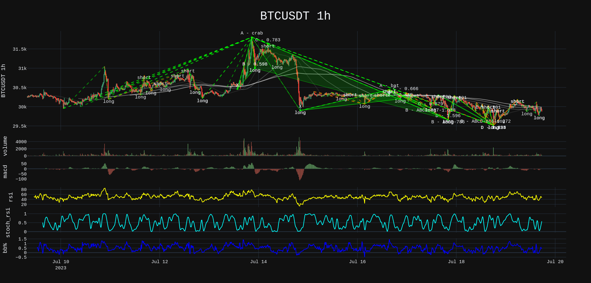
See all harmonic patterns.

>>> p = Plotter(t, 'BTCUSDT', b.HOUR_1)
>>> p.add_matrix_plots(m.get_patterns())
>>> p.show()

You will see something like this.

See all forming patterns.

>>> m = MatrixSearch(t)
>>> m.forming()
>>> p = Plotter(t, 'BTCUSDT', b.HOUR_1)
>>> p.add_matrix_plots(m.get_patterns(formed=False))
>>> p.show()

Position add_matrix_plots

>>> m = MatrixSearch(t)
>>> m.search()
>>> patterns = m.get_patterns(family=m.XABCD)
>>> pattern = patterns[m.XABCD][0]
>>> # After extracting a pattern in isolation a position can be created.
>>> # Position(pattern, symbol, interval, strike_price, dollar_amount)
>>> position = Position(pattern, 'BTSUSDT', b.HOUR_1, pattern.y[-1], 1000)
>>> p = PositionPlotter(t, position)
>>> p.show()

The most useful plot feature is the position plot.

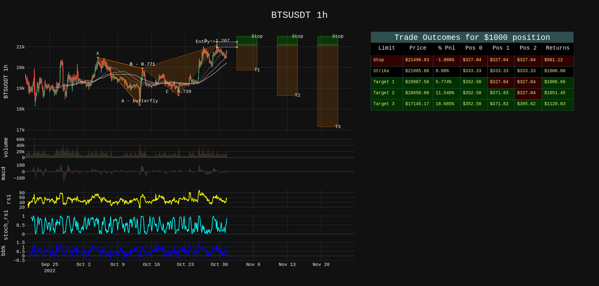
What is the position plot telling?

There is a bearish pattern ( butterfly ). The XAB leg of the price move was a .786 ( in tolerance ) move. The ABC move was between .382 and .886. The final XAD move was 1.27. Sure enough at the price level there was a reaction and so the instruction is to set a price target at the confirmation price level.

The entry or strike price is $21085. If a $1000 dollar amount is entered at this price level then the entire position is divided into 3 even parts.

• Target 1 is usually 50% of the CD leg move.

• The stop should be 1/3 of your target one move.

• Target 2 is the C point on the pattern.

• Target 3 is 1.618 times the cd leg.

The position is divided into 3 parts Pos1 Pos2 Pos3.

1. Pos1, Pos2, Pos3 will all close witha STOP if the price hits 21490 at a loss of -1.88%. This protects your account if the pattern does not play out.

2. Pos1, also close with a LIMIT at $19867 locking in a 21$ profit. Pos2 and pos3 could still stop out but overall you are up $6.66

3. Pos2, can close if the price reaches $18650 BEFORE it hits the STOP price. Pos3 could still stop out leaving you with $51.45 profit.

4. Finally if all 3 targets hit, you make $120 profit on the initial $1000 investment. 12% is not bad.

The %Move column in the plot beside the price column indicates the size of the move. You don’t get 18% profits with that move because you sold out along the way as a risk management strategy.

Call/Put Option Plots

>>> from pyharmonics.marketdata import YahooOptionData
>>> from pyharmonics.plotter import OptionPlotter

>>> yo = YahooOptionData('NVDA')
>>> yo.analyse_options(trend='volume')
>>> p = OptionPlotter(yo, yo.ticker.options[0])
>>> p.show()

>>> yo.analyse_options(trend='openInterest')
>>> p = OptionPlotter(yo, yo.ticker.options[0])
>>> p.show()

The trend or measure for your options activity can be volume or openInterest. The OptionPlotter takes a YahooOptionsData object and an expiry date for any plot.

Although the expiry dates are present in the YahooOptionsData object you must specifically select one to view.

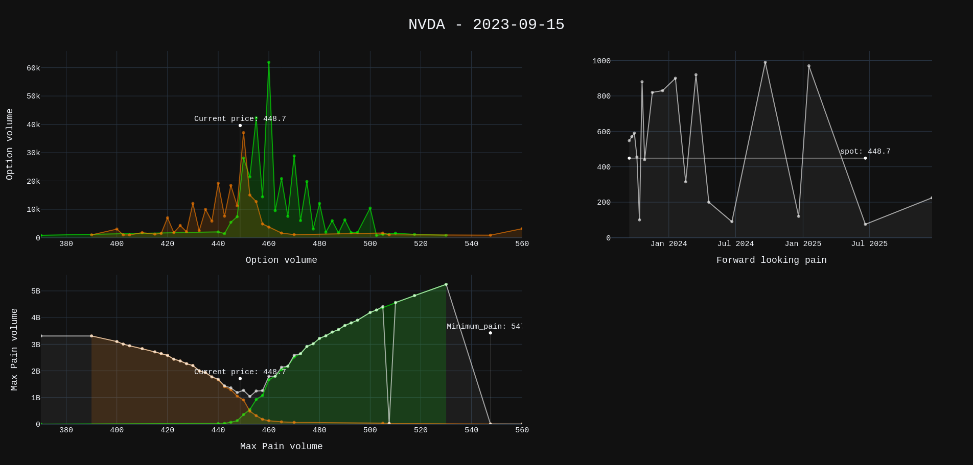
Note

volume or openInterest data resets daily. No activity for a trading can present false points of mimimum pain. Option plots are most complete by end of trading day (usually 16:30 EST)